ISCAN Tutorials

The ISCAN system is a system for going from a raw speech corpus to a data file (CSV) ready for further analysis (e.g. in R), which conceptually consists of a pipeline of four steps:

1. Importing the corpus into ISCAN

   Result: a structured database of linguistic objects (words, phones, sound files).

2. Enriching the database

   Result: Further linguistic objects (utterances, syllables), and information about objects (e.g. speech rate, word frequencies).

3. Querying the database

   Result: A set of linguistic objects of interest (e.g. utterance-final word-initial syllables),

4. Exporting the results

   Result: A CSV file containing information about the set of objects of interest

Preliminaries

Access

Before you can begin the tutorial, you will need access to log in to the ISCAN server via your web browser. To log in to the McGill ISCAN server via your web browser visit https://roquefort.linguistics.mcgill.ca, press the ‘Log in’ button on the top right of the screen and enter the username and password provided.

NWAV 2018 Workshop: the workshop organizers will give you a username and password.

After NWAV 2018 Workshop: Please contact savanna.willerton@mail.mcgill.ca to request access to one of the ISCAN tutorial accounts.

Questions, Bugs, Suggestions

If at any point while using ISCAN you get stuck, have a question, encounter a bug (like a button which doesn’t work), or you see some way in which you believe the user interface could be improved to make usage more clear/smooth/straightforward/etc, then please file an issue on the ISCAN GitHub repository.

There is also a Slack channel you can join if you have quick questions or would like real-time help. Please contact savanna.willerton@mail.mcgill.ca for access.

Dataset

These tutorials use a tutorial corpus, which is (as of Oct 15, 2018) a small subset of ICE-Canada containing speech from all “S2A” files (two male Canadian English speakers). These files can be downloaded from the ICE Canada site, but doing so is not necessary for these tutorials!

Tutorial 1: Polysyllabic shortening

Motivation

Polysyllabic shortening refers to the “same” rhythmic unit (syllable or vowel) becoming shorter as the size of the containing domain (word or prosodic domain) increases. Two classic examples:

• English: stick, sticky, stickiness (Lehiste, 1972)
• French: pâte, pâté, pâtisserie (Grammont, 1914)

Polysyllabic shortening is often – but not always – defined as being restricted to accented syllables. (As in the English, but not the French example.) Using ISCAN, we can check whether a simple version of polysyllabic shortening holds in the tutorial corpus, namely:

• Considering all utterance-final words, does the initial vowel duration decrease as word length increases?

Step 1: Import

This tutorial will use the tutorial corpus available for you, available under the title ‘iscan-tutorial-X’ (where X is a number). The data for this corpus was parsed using the Montreal Forced Aligner, with the result being one Praat TextGrid per sound file, aligned with word and phone boundaries. These files are stored on a remote server, and so do not require you to upload any audio or TextGrid files.

The first step of this analysis is to create a Polyglot DB object of the corpus which is suitable for analysis. This is performed in two steps:

• Importing the dataset using ISCAN, using the phone, word, and speaker information contained in the corpus
• Enriching the dataset to include additional information about (e.g., syllables, utterances), as well as properties about these objects (e.g., speech rate)

To import the corpus into ISCAN, select ‘iscan-tutorial-x’ corpus (replacing “x” with the number you’re using) from the dropdown menu under the ‘Corpora’ tab in the navigation bar. Next, click the ‘Import’ button. This will import the corpus into ISCAN and return a structured database of objects: words, phones, and sound files), that will be interacted with in the following steps.

Step 2: Enrichment

Now that the corpus has been imported as a database, it is now necessary to enrich the database with information about linguistic objects, such as word frequency, speech rate, vowel duration, and so on. You can see the Enrichment page to learn more about what enrichments are possible, but in this tutorial we will just use a subset.

First, select the ‘iscan-tutorial-x’ under the ‘Corpora’ menu, which presents all of the current information available for this specific corpus. To start enrichment, click the ‘create, edit, and run enrichments’ button. This page is referred to as the Enrichment view. At first, this page will contain an empty table - as enrichments are added, this table will be populated to include each of these enrichment objects. On the right hand side of the page are a list of new enrichments that can be created for this database.

Here, we will walk through each enrichment that is necessary for examining vowel duration to address our question (“Considering all utterance final…”).

Syllables

Syllables are encoded in two steps. First, the set of syllabic segments in the phonological inventory have to be specified. To encode the syllabic segments:

1. Select ‘Phone Subset’ button under the ‘Create New Enrichments’ header
2. Select the ‘Select Syllabics’ preset option
3. Name the environment ‘syllabics’
4. Select ‘Save subset’

This will return you to the Enrichment view page. Here, press the ‘Run’ button listed under ‘Actions’. Once syllabic segments have been encoded as such, you can encode the syllables themselves.

1. Under the ‘Annotation levels’ header, press the ‘Syllables’ button
2. Select Max Onset from the Algorithm dropdown menu
3. Select syllabics from the Phone Subset menu
4. Name the enrichment ‘syllables’
5. Select ‘Save enrichment’

Upon return to the Enrichment view, hit ‘Run’ on the new addition to the table.

Speakers

To enrich the database with speaker information:

1. Select the ‘Properties from a CSV’ option
2. Select ‘Speaker CSV’ from the ‘Analysis’ dropdown menu. The CSV for speaker information is available for download.
3. Upload the tutorial corpus ‘speaker_info.csv’ file from your local machine.
4. Select ‘Save Enrichment’ and then ‘Run’ from the Enrichment view.

Lexicon

As with the speaker information, lexical information can be uploaded in an analogous way. Download the Lexicon CSV, for the tutorial corpus, select ‘Lexicon CSV’ from the dropdown menu, save the enrichment, and run it.

Utterances

For our purposes, we define an utterance as a stretch of speech separated by pauses. So now we will specify a minimum duration of pause that separates utterances (150ms is typically a good default).

First, select ‘pauses’ from ‘Annotation levels’, and select ‘<SIL>’ as the unit representing pauses. As before, select ‘Save enrichment’ and then ‘run’.

With the positions of pauses encoded, we are now able to encode information about utterances:

1. Under the ‘Annotation levels’ header, select ‘utterances’.
2. Name the new addition ‘utterance’
3. Enter 150 in the box next to ‘Utterance gap(ms)’
4. Select ‘Save enrichment’, and then ‘Run’ in the Enrichment view.

Speech rate

To encode speech rate information, select ‘Hierarchical property’ from the Enrichment view. This mode allows you to encode rates, counts or positions, based on certain hierarchical properties (e.g., utterances, words). (For example: number of syllables in a word; Here select the following attributes:

1. Enter “speech_rate” as the property name
2. From the Property type menu, select rate
3. From the Higher annotation menu, select utterance
4. From the Lower annotation menu, select syllable

And then, as with previous enrichments, select ‘Save enrichment’ and then run.

Stress

Finally, to encode the stress position within each word:

• Select ‘Stress from word property’ from the Enrichment view menu.
• From the ‘wordproperty’ dropdown box, select ‘stress_pattern’.
• Select ‘Save enrichment’ and run the enrichment in the Enrichment view.

Step 3: Query

Now that the database has been enriched with all of the properties necessary for analysis, it is now necessary to construct a query. Queries enable us to search the database for particular set of linguistic objects of interest.

First, return to the Corpus Summary view by selecting ‘iscan-tutorial-x’ from the top navigation header. In this view, there is a series of property categories which you can navigate through to add filters to your search.

In this case, we want to make a query for:

• Word-initial stressed syllables
• only in words at the end of utterances (fixed prosodic position)

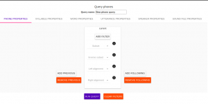
Here, find the selection titled ‘Syllables’ and select ‘New Query’. To make sure we select the correctly positioned syllables, apply the following filters:

Under syllable properties:

• Left aligned with: word
• Under ‘add filter’, select ‘stress’ from the dropdown box, and enter ‘1’ in the text box. This will only select syllables with primary stress in this position.

Under word properties:

• Right aligned with: utterance

Warning

Note that if right alignment with utterances is specified for syllables in this query, this will inadvertently restrict the query to monosyllabic words, as aligning with a higher linguistic type (in this case, utterances) implicitly aligns it to an intermediate linguistic type (in this case, words).

Provide a name for this query (e.g., ‘syllable_duration’) and select ‘Save and run query’.

Step 4: Export

This query has found all word-initial stressed syllables for words in utterance-final position. We now want to export information about these linguistic objects to a CSV file. We want it to contain everything we need to examine how vowel duration (in seconds) depends on word length. Here we may check all boxes which will be relevant to our later analysis to add these columns to our CSV file. The preview at the bottom of the page will be updated as we select new boxes:

1. Under the SYLLABLE label, select:

   • label
   • duration

2. Under the WORD label, select:

   • label
   • begin
   • end
   • num_syllables
   • stress_pattern

3. Under the UTTERANCES label, select:

   • speech_rate

4. Under the SPEAKER label, select:

   • name

5. Under the SOUND FILE label, select:

   • name

Once you have checked all relevant boxes, select ‘Export to CSV’. Your results will be exported to a CSV file on your computer. The name will be the one you chose to save plus “export.csv”. In our case, the resulting file will be called “syllable_duration export.csv”.

Examining & analysing the data

Now that the CSV has been exported, it can be analyzed to address whether polysyllabic shortening holds in the tutorial corpus. This part does not involve ISCAN, so it’s not necessary to actually carry out the steps below unless you want to (and have R installed and are familiar with using it).

In R, load the data as follows:

library(tidyverse)
dur <- read.csv('syllable_duration export.csv')

You may need to first install the tidyverse library using install.packages('tidyverse'). If you are unable to install tidyverse, you may also use library(ggplot2) instead (note: if you do this, please use subset() instead of filter() for the remaining steps).

First, by checking how many word (types) there are for each number of syllables in the CSV, we can see that only 1 word has 4 syllables:

group_by(dur, word_num_syllables) %>% summarise(n_distinct(word_label))

#       word_num_syllables `n_distinct(word_label)`
#                <int>                    <int>
# 1                  1                      109
# 2                  2                       34
# 3                  3                        7
# 4                  4                        1

We remove the word with 4 syllables, since we can’t generalize based on one word type:

dur <- filter(dur, word_num_syllables < 4)

Similarly, it is worth checking the distribution of syllable durations to see if there are any extreme values:

ggplot(dur, aes(x = syllable_duration)) +
geom_histogram() +
xlab("Syllable duration")

As we can see here, there is one observation which appears to be some kind of outlier, which perhaps are the result of pragmatic lengthening or alignment error. To exclude this from analysis:

dur <- filter(dur, syllable_duration < 0.6)

Plot of the duration of the initial stressed syllable as a function of word duration (in syllables):

ggplot(dur, aes(x = factor(word_num_syllables), y = syllable_duration)) +
geom_boxplot() +
xlab("Number of syllables") + ylab("Syllable duration") +
scale_y_sqrt()

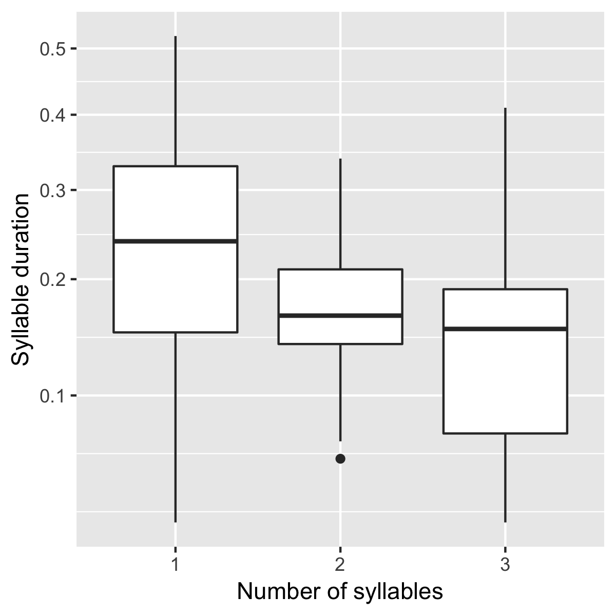
Here it’s possible to see that there is a consistent shortening effect based on the number of syllables in the word, where the more syllables in a word the shorter the initial stressed syllable becomes.

Tutorial 2: Vowel formants

Vowel quality is well known to vary according to a range of social and linguistic factors (Labov, 2001). The precursor to any sociolinguistic and/or phonetic analysis of acoustic vowel quality is the successful identification, measurement, extraction, and visualization of the particular vowel variables for the speakers under consideration. It is often useful to consider vowels in terms of their overall patterning together in the acoustic vowel space.

In this tutorial, we will use ISCAN to measure the first and second formants for the two speakers in the tutorial corpus, for the following vowels (keywords after Wells, 1982): FLEECE, KIT, FACE, DRESS, TRAP/BATH, PRICE, MOUTH, STRUT, NURSE, LOT/PALM, CLOTH/THOUGHT, CHOICE, GOAT, FOOT, GOOSE. We will only consider vowels whose duration is longer than 50ms, to avoid including reduced tokens. This tutorial assumes you have completed the import and enrichment sections from the previous tutorial, and so will only include the information specific to analysing formants.

Step 1: Enrichment

Stressed vowels

First, the set of stress vowels in the phonological inventory have to be specified. To encode these:

1. Select ‘Phone Subset’ button under the ‘Create New Enrichments’ header
2. Select the ‘Select Stressed Vowels’ preset option
3. Name the environment ‘stressed_vowels’
4. Select ‘Save subset’

This will return you to the Enrichment view page. Here, press the ‘Run’ button listed under ‘Actions’.

Acoustics

Now we will compute vowel formants for all stressed syllables using an algorithm similar to FAVE.

For this last section, you will need a vowel prototype file. For the purposes of this tutorial, the file for the tutorial corpus is provided here:

ISCAN_Prototypes

Please save the file to your computer.

From the Enrichment View, under the ‘Acoustics’ header, select ‘Formant Points’. As usual, this will bring you to a new page. From the Phone class menu, select stressed_vowels. Using the ‘Choose Vowel Prototypes CSV’ button, upload the ICECAN_prototypes.csv file you saved. For Number of iterations, type 3 and for Min Duration (ms) type 50ms.

Finally, hit the ‘Save enrichment’ button. Then click ‘Run’ from the Enrichment View.

Step 2: Query

The next step is to search the dataset to find a set of linguistic objects of interest. In our case, we’re looking for all stressed vowels, and we will get formants for each of these. Let’s see how to do this using the Query view.

First, return to the ‘iscan-tutorial-x’ Corpus Summary view, then navigate to the ‘Phones’ section and select New Query. This will take you to a new page, called the Query view, where we can put together and execute searches. In this view, there is a series of property categories which you can navigate through to add filters to your search. Under ‘Phone Properties’, there is a dropdown menu with search options labelled ‘Subset’. Select ‘stressed_vowels’. You may select ‘Add filter’ if you would like to see more options to narrow down your search.

The selected filter settings will be saved for further use. It will automatically be saved as ‘New phone query’, but let’s change that to something more memorable, say ‘Tutorial corpus Formants’. When you are done, click the ‘Save and run query’ button. The search may take a while, especially for large datasets, but should not take more than a couple of minutes for this small subset of the ICE-Can corpus we’re using for the tutorials.

Step 3: Export

Now that we have made our query and extracted the set of objects of interest, we’ll want to export this to a CSV file for later use and further analysis (i.e. in R, MatLab, etc.)

Once you hit ‘Save query’, your search results will appear below the search window. Since we selected to find all stressed vowels only, a long list of phone tokens (every time a stressed vowel occurs in the dataset) should now be visible. This list of objects may not be useful to our research without some further information, so let’s select what information will be visible in the resulting CSV file using the window next to the search view.

Here we may check all boxes which will be relevant to our later analysis to add these columns to our CSV file. The preview at the bottom of the page will be updated as we select new boxes:

Under the Phone header, select:

• label
• begin
• end
• F1
• F2
• F3
• B1 (The bandwidth of Formant 1)
• B2 (The bandwidth of Formant 2)
• B3 (The bandwidth of Formant 3)
• num_formants

Under the Syllable header, select:

• stress
• position_in_word

Under the Word header, select:

• label
• stress_pattern

Under the Utterance header, select:

• speech_rate

Under the Speaker header, select:

• name

Under the Sound File header, select:

• name

Once you have checked all relevant boxes, select ‘Export to CSV’. Your results will be exported to a CSV file on your computer. The name will be the one you chose to save plus “export.csv”. In our case, the resulting file will be called “Tutorial Formants export.csv”.

Step 4. Examining & analysing the data

With the tutorial complete, we should now have a CSV file saved on our personal machine containing information about the set of objects we queried for and all other relevant information.

We now examine this data. This part doesn’t use ISCAN, so it’s not necessary to actually carry out the steps below unless you want to.

In R, load the data as follows:

library(tidyverse)
v <- read.csv("Tutorial Formants export.csv")

Rename the variable containing the vowel labels to ‘Vowel’, and reorder the vowels so that they pattern according to usual representation in acoustic/auditory vowel space:

v$Vowel <- v$phone_label
v$Vowel = factor(v$Vowel, levels = c('IY1', 'IH1', 'EY1', 'EH1', 'AE1', 'AY1','AW1', 'AH1', 'ER1', 'AA1', 'AO1', 'OY1', 'OW1', 'UH1', 'UW1'))

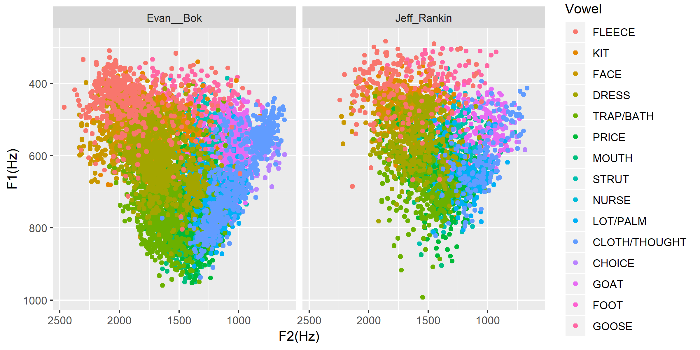
Plot the vowels for the two speakers in this sound file:

ggplot(v, aes(x = phone_F2, y = phone_F1, color=Vowel)) +
geom_point() +
facet_wrap(~speaker_name) +
scale_colour_hue(labels = c("FLEECE", "KIT", "FACE", "DRESS", "TRAP/BATH", "PRICE", "MOUTH", "STRUT", "NURSE", "LOT/PALM", "CLOTH/THOUGHT", "CHOICE", "GOAT", "FOOT", "GOOSE")) +
scale_y_reverse() +
scale_x_reverse() +
xlab("F2(Hz)") +
ylab("F1(Hz)")

Tutorial 3: Sibilants

Sibilants, and in particular, /s/, have been observed to show interesting sociolinguistic variation according to a range of intersecting factors, including gendered, class, and ethnic identities (Stuart-Smith, 2007; Levon, Maegaard and Pharao, 2017). Sibilants - /s ʃ z ʒ/ - also show systematic variation according to place of articulation (Johnson, 2003). Alveolar fricatives /s z/ as in send, zen, are formed as a jet of air is forced through a narrow constriction between the tongue tip/blade held close to the alveolar ridge, and the air strikes the upper teeth as it escapes, resulting in high pitched friction. The post-alveolar fricatives /ʃ ʒ/, as in ‘sheet’, ‘Asia’, have a more retracted constriction, the cavity in front of the constriction is a bit longer/bigger, and the pitch is correspondingly lower. In many varieties of English, the post-alveolar fricatives also have some lip-rounding, reducing the pitch further.

Acoustically, sibilants show a spectral ‘mountain’ profile, with peaks and troughs reflecting the resonances of the cavities formed by the articulators (Jesus and Shadle, 2002). The frequency of the main spectral peak, and/or main area of acoustic energy (Centre of Gravity), corresponds quite well to shifts in place of articulation, including quite fine-grained differences, such as those which are interesting for sociolinguistic analysis: alveolars show higher frequencies, more retracted post-alveolars show lower frequencies.

As with the previous tutorials, we will use ISCAN to select all sibilants from the imported sound file for the two speakers in the tutorial corpus, and take a set of acoustic spectral measures including spectral peak, which we will then export as a CSV, for inspection.

Step 1: Enrichment

It is not necessary to re-enrich the corpus with the elements from the previous tutorial, and so here will only include the enrichments necessary to analyse sibilants.

Sibilants

Start by looking at the options under ‘Create New Enrichments’, press the ‘Phone Subset’ button under the ‘Subsets’ header. Here we select and name subsets of phones. If we wish to search for sibilants, we have two options for this corpus:

• For our subset of ICE-Can we have the option to press the pre-set button ‘Select sibilants’.
• For some datasets the ‘Select sibilants’ button will not be available. In this case you may manually select a subset of phones of interest.

Then choose a name for the subset (in this case ‘sibilants’ will be filled in automatically) and click ‘Save subset’. This will return you to the Enrichment view where you will see the new enrichment in your table. In this view, press ‘Run’ under ‘Actions’.

Acoustics

For this section, you will need a special praat script saved in the MontrealCorpusTools/SPADE GitHub repository which takes a few spectral measures (including peak and spectral slope) for a given segment of speech. With this script, ISCAN will take these measures for each sibilant in the corpus. A link is provided below, please save the sibilant_jane_optimized.praat file to your computer: Praat script

From the Enrichment View, press the ‘Custom Praat Script’ button under the ‘Acoustics’ header. As usual, this will bring you to a new page. First, upload the saved file ‘sibilant_jane_optimized.praat’ from your computer using ‘Choose Praat Script’ button. Under the Phone class dropdown menu, select sibilant.

Finally, hit the ‘Save enrichment’ button, and ‘Run’ from the Enrichment View.

Hierarchical Properties

Next, from the Enrichment View press the ‘Hierarchical property’ button under ‘Annotation properties’ header. This will bring you to a page with four drop down menus (Higher linguistic type, Lower linguistic type, Subset of lower linguistic type, and Property type) where we can encode speech rates, number of syllables in a word, and phone position.

While adding each enrichment below, remember to choose an appropriate name for the enrichment, hit the ‘save enrichment’ button, and then click ‘Run’ in the Enrichment View.

Syllable Count 1 (Number of Syllables in a Word)

1. Enter “num_syllables” as the property name
2. From the Property type menu, select count
3. From the Higher annotation menu, select word
4. From the Lower annotation menu, select syllable

Syllable Count 2 (Number of Syllables in an Utterance)

1. Enter “num_syllables” as the property name
2. From the Property type menu, select count
3. From the Higher annotation menu, select utterance
4. From the Lower annotation menu, select syllable

Phone Count (Number of Phones per Word)

1. Enter “num_phones” as the property name
2. From the Property type menu, select count
3. From the Higher annotation menu, select word
4. From the Lower annotation menu, select phone

Word Count (Number of Words in an Utterance)

1. Enter “num_words” as the property name
2. From the Property type menu, select count
3. From the Higher annotation menu, select utterance
4. From the Lower annotation menu, select word

Phone Position

1. Enter “position_in_syllable” as the property name
2. From the Property type menu, select position
3. From the Higher annotation menu, select syllable
4. From the Lower annotation menu, select phone

Step 2: Query

The next step is to search the dataset to find a set of linguistic objects of interest. In our case, we’re looking for all sibilants. Let’s see how to do this using the Query view.

First, return to the ‘iscan-tutorial-X’ Corpus Summary view, then navigate to the ‘Phones’ section and select New Query. This will take you to a new page, called the Query view, where we can put together and execute searches. In this view, there is a series of property categories which you can navigate through to add filters to your search. Under ‘Phone Properties’, there is a dropdown menu labelled ‘Subset’. Select ‘sibilants’. You may select ‘Add filter’ if you would like to see more options to narrow down your search.

The selected filter settings will be saved for further use. It will automatically be saved as ‘New phone query’, but let’s change that to something more memorable, say ‘SibilantsTutorial’. When you are done, click the ‘Run query’ button. The search may take a while, especially for large datasets.

Step 3: Export

Now that we have made our query and extracted the set of objects of interest, we’ll want to export this to a CSV file for later use and further analysis (i.e. in R, MatLab, etc.)

Once you hit ‘Run query’, your search results will appear below the search window. Since we selected to find all sibilants only, a long list of phone tokens (every time a sibilant occurs in the dataset) should now be visible. This list of sibilants may not be useful to our research without some further information, so let’s select what information will be visible in the resulting CSV file using the window next to the search view. G Here we may check all boxes which will be relevant to our later analysis to add these columns to our CSV file. The preview at the bottom of the page will be updated as we select new boxes:

Under the Phone header, select:

• label
• begin
• end
• cog
• peak
• slope
• spread

Under the Syllable header, select:

• stress

Under the Word header, select:

• label

Under the Utterance header, select:

• speech_rate

Under the Speaker header, select:

• name

Under the Sound File header, select:

• name

Once you have checked all relevant boxes, click the ‘Export to CSV’ button. Your results will be exported to a CSV file on your computer. The name will be the one you chose to save for the Query plus “export.csv”. In our case, the resulting file will be called “SibilantsTutorial export.csv”.

Step 4: Examining & analysing the data

With the tutorial complete, we should now have a CSV file saved on our personal machine containing information about the set of objects we queried for and all other relevant information.

We now examine this data. This part doesn’t use ISCAN, so it’s not necessary to actually carry out the steps below unless you want to.

First, open the CSV in R:

s <- read.csv("SibilantsTutorial export.csv")

Check that the sibilants have been exported correctly:

levels(s$phone_label)

Change the column name to ‘sibilant’:

s$sibilant <- s$phone_label

Check the counts for the different voiceless/voiced sibilants - /ʒ/ is rare!

summary(s$sibilant)

# S   SH    Z     ZH
# 2268  187 1296  3

Reorder the sibilants into a more intuitive order (alveolars then post-alveolars):

s$sibilant <- factor(s$sibilant, levels = c('S', 'Z', 'SH', 'ZH'))

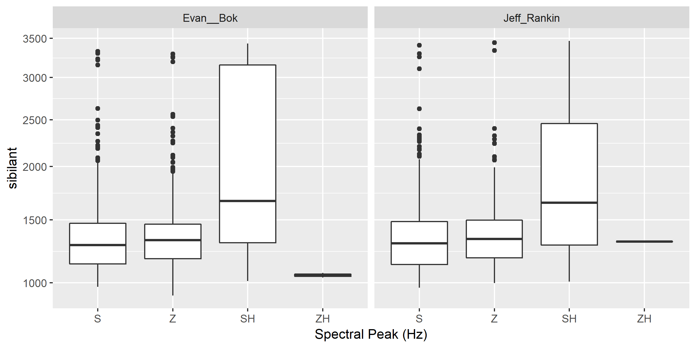
Finally, plot the sibilants for the two speakers:

ggplot(s, aes(x = factor(sibilant), y = phone_peak)) +
geom_boxplot() +
xlab("Spectral Peak (Hz)") +
ylab("sibilant") +
scale_y_sqrt() +
facet_wrap(~speaker_name)

Tutorial 4: Custom scripts

Often in studies it is necessary to perform highly specialized analyses. As ISCAN can’t possibly provide every single analysis that anyone could ever want, there is a way to perform analyses outside of ISCAN, and then bring them in. This is the purpose of the ‘Custom Properties from a Query-generated CSV’ enrichment. Using it is relatively straightforward, although it requires some prelimanary steps to get the data in the right format before using. It also requires access to the original sound files of a corpus if you wish to use these in your analysis.

In this tutorial we will be using an R script, but you can use any script or software that you so choose.

Step 1: Necessary Enrichments

The only necessary enrichment to do in this tutorial is to encode a sibilant subset of phones. To do this, start at the ‘iscan-tutorial-X’ corpus summary view, and click on the ‘Create, run and edit enrichments’ button in the centre column. Then, click on ‘Phone Subset’.

At the enrichment page, click on the select sibilants button, then name the subset ‘sibilants’ and save the subset.

Finally, at the main enrichment page, run the sibilant enrichment.

Step 2: Running a phone query

Now that we have all the enrichments we need, we can go to the Query View.

Starting at the ‘iscan-tutorial-X’ corpus summary view, navigate to the phones section of the left-most column and click “new Phone Query”. From there, the you’ll have the option to choose various different filters to select a subset of phones. For this tutorial we’re looking at sibilants, so all you need to do is select the sibilants subset from the first drop-down menu from the centre menu.

Feel free to also re-name the query to anything you’d like, for example ‘sibilant ID query’. From there, click on ‘Run query’ and wait for the query to finish.

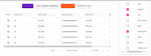
Step 3: Exporting phone IDs

Once the query has finished, a new pane will appear to the right of the window. This pane will contain a list of different properties of the phones found, and properties of the syllables, words, and utterances that a phone is in. These are the columns that will be included in the CSV that you will download from ISCAN.

For the script, we will need a couple different columns.

Under the Phone header, select:

• label
• begin
• end
• id

Under the Sound File header, select:

• name

Once all these columns have been selected, click the “Generate CSV Export File” in the row of buttons in the centre of the screen, above the results of the query. This may take a second or two to run, then once it’s available, click on the “Save CSV export file” and save the file somewhere convenient on your computer.

An important thing to note for this section is that while you can rename columns for export, you should not rename the ID column if you intend on importing this CSV later. By default, a phone ID column will be labeled “phone_id”. When importing, ISCAN looks for a column that ends with “_id” and then uses the first half of the name of that column to know what these IDs represent(in this case, phones). You also should not have multiple ID columns in your import CSV, although if you do, ISCAN will use the first ID column only.

Step 4: Running the R script

The script and associated files can be downloaded here. This script estimates spectral features in R (Reidy, 2015).

In order to get this script running on your computer, you will have to make a few minor edits once you have extracted the ZIP file. Open up ‘iscan-token-spectral-demo.R’ in your text editor.

At the top of the file, there will be two file paths defined. Change ‘sound_file_directory’ to the file path of where you have the sound files of the tutorial corpus. Then, change ‘corpus_directory’ to be the file path of the CSV that you downloaded from ISCAN. I have it as a relative path, but you can of course make it an absolute path.

sound_file_directory <- "/home/michael/Documents/Work/test_corpus"
corpus_data <- read.csv("../sibilants_export.csv")

This script also assumes you have not renamed any of the columns that you exported. If you did change any columns’ name, you will have to look through the script and change the following lines to the names of the corresponding columns.

sound_file <- paste(corpus_data[row, "sound_file_name"], '.wav', sep="")
begin <- corpus_data[row, "phone_begin"]
end <- corpus_data[row, "phone_end"]

Finally, you can run the script in R, and it will create a new CSV file, ‘spectral_sibilants.csv’ that we will import to ISCAN.

Step 4: Importing the CSV

Back in ISCAN, go to the enrichments page for your tutorial corpus.

Under ‘Annotation properties’, click on the ‘Custom Properties from a Query-generated CSV’ button.

From this page, click on the “browse” button and navigate to the ‘spectral_sibilants.csv’ generated in the last step. Select it for upload, then click on “Upload CSV”. This may take a second or two, so be patient.

After this, a new list of properties will appear which come from the columns of the CSV. Scroll down, and select all the features that start with ‘spectral’.

Then, click ‘save enrichment’, and from the main enrichment page, run the enrichment labelled ‘Enrich phone from “spectral_sibilants.csv”’.

Now you’re done! ISCAN will now have all of the values calculated by the R script associated with all the sibilants in the corpus. You can test this out by going to the phone query you created earlier. You should see all these new properties in the column selection pane, although you may need to click “Refresh Query” before the values appear.